


Pseudoatomic resolution in AFM imaging of HOPG
Application Note 079 (pdf 810 Kb)
Baturin A.S., Chuprik A.A.
OVERVIEW
A possible way to achieve atomic resolution in AFM imaging on open air [1, 2] is using of the stick-slip effect (see. 2.6.5 and 4.1 of SPM basics). In this mode, the probe motion is jogging with retardation in minima of the interaction potential that correspond to atoms of the atomic surface. This jogging, however, is smoothed by capillary forces due to the adsorbate film on the sample surface that is unavoidable in open-air scans. So, the image contrast lowers and it can be insufficient to achieve the atomic scale resolution.
A proper material to achieve the atomic resolution is highly oriented pyrolytic graphite (HOPG). First, it is hydrophobic, and so the adsorbate film is very thin or even absent; second, the procedure on HOPG cleaving is very convenient.
Notice that the term atomic resolution is not quite correct when applied to the lateral force technique. Although the distribution of the friction force strictly correlates with the crystalline potential of the sample, the detected maxima are shifted relative to atoms positions which define the surface landscape [3]. That is why we prefer to use further the term pseudoatomic resolution in discussion of the technique.
PREPARING THE SAMPLE
- Fix the sample on the substrate with a double-sided sticky tape.
- Prepare a fresh cleavage of HOPG surface. To this purpose, take a small piece of sticky tape, paste it on the graphite surface, and smooth it out carefully to remove any air bubbles. Then remove the piece of sticky tape with the upper layer of graphite. This results in atomic smoothing of the sample surface. Quality of the cleavage depends on the direction the piece of sticky tape was removed. For better results, it is recommended to use the removal angle that provides the smoothest surface.
SELECTING A CANTILEVER
To achieve the pseudoatomic resolution with HOPG samles, it is recommended to use short rectangular cantilevers of sufficiently high stiffnes that are most sensitive to lateral twisting. The exemplary study below was performed with the silicon cantilever CSC12(A). This cantilever is characterized by the following specifications:
length
width
thickness
stiffness
tip length
tip curvature radius less
l=110 µm
w=35 µm
t=1 µm
l/c=0.95 N/m
ltip=10-15 µm
10 nm
SELECTING A SCAN AREA
- Approach the tip to the surface in the contact mode after selecting the contact mode of operation. Parameters of the mode are: SetPoint=1.5 nA (for the cantilever CSC12(A), this sets the loading force to 17 nN), feedback gain FB Gain=0.7.
- Select an area of 3x3 µm size. Scan it in the constant force mode.
- Find an atomically smooth (free of atomic steps) region of approximate size 6х6 nm in the collected image (see Fig. 1) for further investigation.
Fig. 1. Graphite surface image collected with the constant force technique. Scan area 3x3 µm (a).
Landscape along the white line section (b).
ESTIMATING RELEVANT INSTRUMENTAL PARAMETERS
- Collect the spectroscopy DFL(z) that is the relation of the DFL signal (in nA) to the vertical displacement of the sample z (in nm) (see Fig. 2). This relation provides estimation of the calibrating constant b, to calculate the vertical displacement (in nm) of the cantilever by the DFL signal (in nA). The constant depends on the construction of the detecting optical system, electronic amplifying circuitry of signals from photosensors, and the cantilever length.
Fig. 2. Spectroscopy DFL(z)
- Estimate the slope of the left part of the plot b=ΔDFL/Δz [nA/nm]. This inclined segment corresponds to the tip-sample contact. In our example, b=0.086&bsp;nA/nm.
- By the manufacturer specification of the cantilever stiffness l/c (in nN/nm), calculate the scaling ratio of the vertical load [nN] from DFL [nA] according to:
 [nA/nN]. In our example, a=0.091 nA/nN.
SETTING THE LOADING
- The DFL signal contains a certain contribution of the vertical loading F2 (see Fig. 3) that relates to the landscape in the constant height mode as ΔF2=Δh/c, as well as a contribution of the longitudinal friction force Fy=µFz ( µ being the friction coefficient, see Fig. 4):
where czy - zy is the zy component of the inverse stiffness tensor (see formula in section 2.1.3).

Fig. 3. Vertical z-type bend
Fig. 4. Vertical z-type bend
- The relations above provide:

- The only controllable parameter is the load F2. If it is small, the DFL signal follows the sample landscape (see the first term). If it is large, the second term dominates and variation of the friction coefficient defines the signal.
- As the pseudoatomic resolution needs to use the longitudinal friction force, we have to choose the load F2 so that the first contribution in DFL does not affect the image contrast.
- The loading level is defined through the SetPoint parameter that is measured in nA. With the selected cantilever CSC12(А), it is recommended to take F2 in the range 80÷350 nN that is equivalent to 7÷30 nA for SetPoint. Lower values are insufficient for the pseudoatomic resolution (see Fig. 5a) while larger values may result in destruction of the sample and vanishing of the image contrast (see Fig. 5c). Notice that distinctiveness of the atomic image collected with the LF signal is virtually independent of the loading taken at those levels.
Fig. 5a. Distribution of the DFL signal at SetPoint=6 nA

Fig. 5b. Distribution of the DFL signal at SetPoint=17 nA
Fig. 5c. Distribution of the DFL signal at SetPoint=30 nA
SCANNING
- After setting the SetPoint parameter to define the load, select the constant height mode. The results below correspond to the load 190 nN (i.e. SetPoint=17 nA). In the course of scanning, the load slightly variates due to the landscape
 .
. - Click the Settings button to select signals DFL и LAT(LF) to be recorded under scanning.
- Select a direction perpendicular to the cantilever axis to be the scanning direction: HBL or HBR for pseudoatomic resoulution with the signal LF; VBL for pseudoatomic resoulution with the signals DFL and LF (see "Stick-slip motion on the nanoscale").
- Select the maximum available scanning speed.
- Select the image size 256x256.
- Perfom scanning. The image should look like:
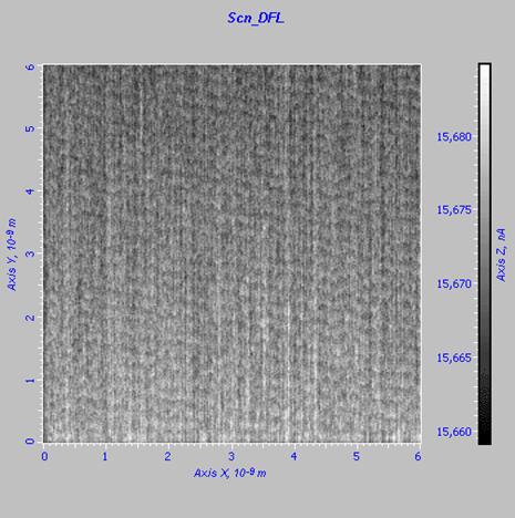
Fig. 6а. Distribution of the DFL signal
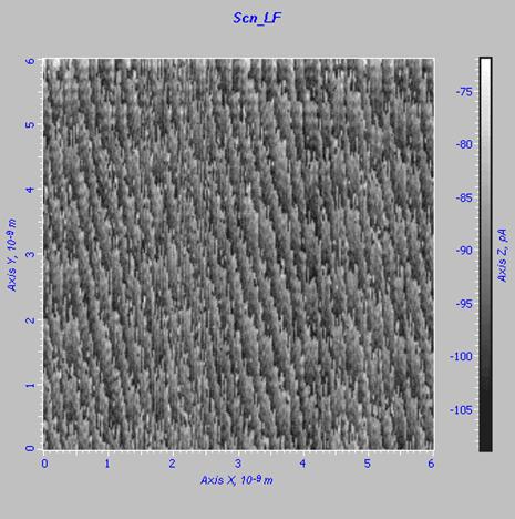
FIg. 6b. Distribution of the LF(LAT) signal
PROCESSING IMAGES
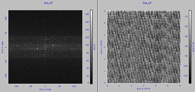
The collected image of the crystal lattice suffers from the noise. To improve quality of the image, i.e. to eliminate noises, we use the Fourier-filtering technique.
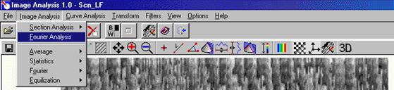
- Select the desired image, e.g. the distribution of the распределение сигнала LF (LAT) signal.
- Click the
 , button at the top of the right panel and select the Image Analysis item:
- This opens the Image Analysis window. Select the Image Analysis -> Fourier Analysis menu command in this window:
-
The program produces the Fourier image of the scan:
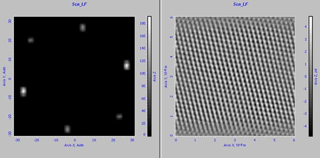
- Now we are cleaning the noise from the image spectrum. Click the
 button (Select Region) in the Toolbar. This tool serves for zeroing values in a rectangle. After zeroing the selected region of the spectrum, the filtered image is calculated and displayed. Obtain an image like this:
- Repeat steps 1–4 for the image with the DFL signal:
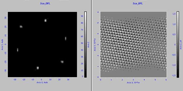
- The final images should be like those below:
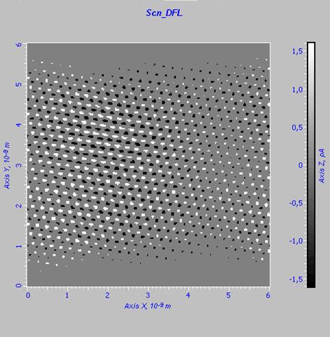
Fig. 7a. Fourier-filtered image of the DFL signal distribution
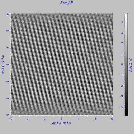
Fig. 7b. Fourier-filtered image of the LF(LAT) signal distribution
CONCLUSION
Demonstration of the pseudoatomic resolution in AFM imaging on open air is performed conveniently with a testing HOPG sample. The measurement procedure needs to use a sufficiently stiff and short cantilever and to define the load so that the pseudoatomic resolution was achieved both with the LAT signal distribution and with the DFL signal distribution, with the sample remaining non-destructed. The imaging quality improves with the use of Fourier filtering, the option available in the Control Program of the microscope.
REFERENCES
- Sasaki N., Kobayashi K., Tsukada M., Phys. Rev. B 54, N3 (1996) 2138-2149.
- Handbook of Micro/Nanotribology / Ed. by Bhushan Bharat. - 2d ed. - Boca Raton etc.: CRC press, 1999.
- N.P. D’Costa, J.H. Hoh, Rev. Sci.Instrum. 66 (1995) 5096-5097.