


2.6.6 Stick-slip phenomenon on the microscale
Introduction.
In microtribology, the friction is considered on the continuum scale and against nanotribology, the atomic structure of matter is not taken into account. The effective contact area in microtribology is about 100 nm so thousands of atoms participate in molecular interaction. The lattice potential periodic character which plays an important role on the nanoscale, becomes inessential in microtribology because potential features are indistinguishable on this scale.
Our goal is to construct a theoretical friction model on the microscale and creation of the computing algorithm (scheme). In a built-up program based on this one-dimensional numerical model you can change parameters and watch changes in the frictional force during scanning.
We are not going to solve an accurate quantitative problem predicting experimental results but construct a principal model which explains the character of motion, in particular, the so called "stick-slip" motion. Therefore, values of some parameters will be introduced without theoretical substantiation but for the sake of adequacy of obtained results.
As a model object we take a flat sample and a probe in contact with it. The scanning is performed in a contact mode in the direction normal to a cantilever axis.
Fig. 1. Cantilever model.
Cantilever (or, rather, its tip) is modeled by a linear two-dimensional damped oscillator (Fig. 1). Because we construct the one-dimensional model and scanning is performed in the lateral direction, we shall consider only tip side deflections which are determined mainly by torsion deformation (see chapter 2.1.4). The cantilever is described in this case by three parameters: torsional stiffness
 , damping factor in a given direction
 , and oscillator effective mass
 .
.
Cantilever torsional stiffness can be calculated basing on its geometry (see chapter 2.1.4). The mass is determined from the relation

(1)
where
 – first mode frequency of torsional oscillations.
For the damping factor we can take the value obtained from the Q-factor of these oscillations
 :
:

(2)
Physical fundamentals of the model.
While moving along the sample surface, the cantilever experiences an adhesive attraction. In this model, the origin of this interaction is not discussed and its character is just postulated. The nature of adhesion can be different – from interdiffusion of long organic molecules to capillary effect of adsorbed films. The force of adhesion can vary from some minimal value
 to maximal
 . Introduced is the relaxation time
 during which the attraction force on the immovable tip after contact increases from
to
[1]:
during which the attraction force on the immovable tip after contact increases from
to
[1]:
(3)
In other words, the longer the cantilever is located at a given site, the more it is "stuck". Due to postulating of such kind of friction, arises a non-trivial stick-slip phenomenon that will be discussed later.
Let us introduce such a notion as "contact age"
 – effective time of the tip being in contact at given point. The contact age (by definition) is given by integral:
(4)
In this formula
 – function describing the position (coordinate) of the tip during scanning at preceding moments of time. Integration is performed from the contact onset to the current moment. Effective radius of interaction
 is the distance which the clamped cantilever end must move to break the contact between the tip and the surface. Although the contact age depends on all the previous scan history, due to the exponent presence only those moments of time when the tip is in the
-vicinity of the given point contribute sufficiently into the integral. Thus, when the cantilever is far from the studied vicinity, the time is "forgotten".
is the distance which the clamped cantilever end must move to break the contact between the tip and the surface. Although the contact age depends on all the previous scan history, due to the exponent presence only those moments of time when the tip is in the
-vicinity of the given point contribute sufficiently into the integral. Thus, when the cantilever is far from the studied vicinity, the time is "forgotten".
Naturally, for a motionless tip, the contact age is equal to the time that passed from the moment of the contact onset. If the tip moves across the sample uniformly with velocity
 , the contact age is the same in all sites and equal to

(5)
Equations of the model.
The tip move obeys the second Newton law [1,5]:
(6)
where
 depends on contact age (4) as follows:
(7)
The left hand side includes the cantilever natural elastic force, arising from the probe deflection from the non-deformed position
 during scanning, and the damping. The external force represented by the equation right hand side is the microscopic frictional force considered above.
Set of equations (6) and (7) describe the constructed model completely. For the numerical system construction it is convenient to replace integral equation (4) with equivalent differential one:

(8)
To solve system (6-7) numerically, it is brought to the system of three differential equations, then the explicit scheme is utilized.
Stick-slip phenomenon.
In the constructed model, a sticking-sliding phenomenon, which reflects the saw-tooth behavior of the frictional force in time, can become apparent at certain parameters. For the equations set (6-7) there is the solution instability with respect to small perturbations. The characteristic profile of the frictional force during the unstable motion is depicted in Fig. 2 [1-5]. This is the stick-slip motion: the probe is held at certain sites, the frictional force starts to raise until the probe separation occurs and the frictional force jumps to a certain minimum.
Fig. 2. Plot of frictional force vs. time.
The spectral analysis of the linear stability of the model nonlinear equations set allows to determine the critical relationship between problem parameters at which the motion character changes from stable to irregular stick-slip:
(9)
It is important that the character of motion – stable or unstable – depends on scan speed. There exists a certain critical speed
 below which the uniform sliding transforms into stick-slip. The red curve
 in the parameters plane
 at the other parameters being fixed, demarcates the regions of stable and unstable motion.
Fig. 3. Regions of stable and stick-slip motion.
The plot permits to draw a conclusion that for any stiffness
there is a certain speed
over which no stick-slip occurs. Note that there is the maximum speed
 at which (if extremely "soft" cantilever is chosen:
 ) the stick-slip motion is available.
Expression (4) contains, however, the other model parameters. It is important to discuss how they affect the instability onset. Upon variation of relaxation time
, interaction radius
, and force change
 , the critical curve
in Fig. 3 will shift. One can show that if the following inequality is satisfied
, the critical curve
in Fig. 3 will shift. One can show that if the following inequality is satisfied

(10)
the region of unstable motion in the plot disappears. This means that at any scan speed the sliding is uniform. Therefore, to reach the stick-slip motion, it is not enough to adjust the speed but it is necessary that relaxation time
and force variation
are large enough while
and
are small.
Features of the model numerical realization.
Examining equation (2) one can easily reveal its limitation. Once in contact with a sample, an immovable probe should start moving due to the frictional force and that is a physical nonsense. Such errors will arise at rest or at very low probe speed. That is why the model includes a kind of "stabilizer", i.e. the frictional force direction is chosen basing on the following criteria:
(11)
Another feature is that the solution has regions of both gradual and sudden change, the last needed small integration step for the correct calculation. To optimize calculations, the algorithm with an adaptive step was implemented. In case of sudden solution change, the step of difference equations integration is halved, otherwise, it is increased.
Choosing the problem parameters.
The cantilever parameters calculation was given above. The other parameters
,
,
,
are chosen empirically so that modeling results are close to experimental. Our goal is not the precise solution of the problem to predict experimental results, but the construction of the principal model explaining stick-slip behavior.
For the majority of materials, the effective sticking (adhesion) radius
should be taken as ~ 0.2 nm and the relaxation time
as ~ 150 ms. In its turn, the minimum force
and force variation
are set taking into account the real friction coefficient of materials and stick-slip appearance.
In the built-in program (see Flash model), the most typical values of listed parameters are set by default which allow to reveal all the microfriction model features:
| velocity | = 5 mm/s |
| scan region |  = 500 nm = 500 nm |
| frequency of first torsional mode (for CSC12(B) cantilever type) |
 = 351.71 kHz = 351.71 kHz |
| effective mass | = 6.72 * 10-12 kg |
| Q-factor | = 10 |
| damping | = 4.91 * 105 1/s |
| minimal force | = 5 * 10-7 N |
| variation of frictional force | = 10 * 10-7 N |
| relaxation time | = 5 ms |
| interaction radius | = 0.2 nm. |
Let us compare the results of numerical modeling and experimantal data. List of parameters for numerical modeling (Fig. 4):
| scan velocity | = 110 mm/s |
| scan region | = 11 mm |
| CSC12(B) cantilever type minimal force |
= 20 mN |
| variation of frictional force | = 50 mN |
| relaxation time | = 5 ms |
| interaction radius | = 0.2 nm. |
Fig. 4. Results of numerical modeling.
List of experimantal parameters (Fig. 5):
| scan velocity | = 110 mm/s |
| scan region | = 11 mm |
| cantilever type | CSC12(B) |
| sample | smooth silicon plate |
| SetPoint = 0.36 nA (squeeze force 2.1 nN) | |
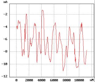
Fig. 5a. Experimantal results.
Scan direction: from left to right.
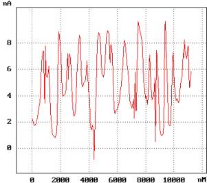
Fig. 5b. Experimantal results.
Scan direction: from right to left.
Friction force can be calculated by means of the formula (1) in chapter 2.6.4:
= 170 nN,
= 500 nN.
In accordance with Fig. 5, if the scan direction changes the signal LAT changes sign on contrary. It means that cantilever twists in different side at opposite scan direction.
A stick-peak period of numerical modeling is in close agreement with experimantal results and approximately equals to ~ 1 mm. However, it should be emphasized that friction force in the numerical model exceeds the experimental condition more than one hundred times.
The built-in program features.
The built-in calculation program allows to set up parameters and obtain the evolution in time of the LAT signal, which is proportional to the friction force, and to see also the contact age at any time. The user can choose any relation to display from the drop-down menu in the top right corner upon calculation completion.
You can change the following model default parameters:
- Cantilever parameters. It is possible to choose between one of the standard cantilevers and "My" cantilever typing dimensions of the latter, its torsional stiffness
, frequency of first torsional mode and effective mass
being calculated automatically.
- Damping
- Minimum frictional force
- Variation of frictional forc
- Relaxation time
- Interaction radius
- Scan velocity
- Scan length
Considering results.
Let us examine a few examples. We shall use the default parameters and change only scan speed and relaxation time.
Case 1.
Parameters:
= 5 ms;
= 5 mm/s;
= 500 nm.
This is a typical stick-slip motion. Parameters point
is in the unstable area of the plot in Fig. 3.
The force (or, rather, LAT signal describing the elastic probe deflection under the influence of the friction) is of the saw-tooth form. The contact age changes non-uniformly, too which is the evidence that the probe jogs staying at sites of sticking.
Case 2.
Parameters:
= 5 ms;
= 5 mm/s;
= 100 nm.
Once started, the probe moves uniformly without stick-slip. At such a small relaxation time
condition (10) of the lack of unstable region in the plot in Fig. 3 is satisfied. This in fact means that during the uniform probe move, the relaxation can occur because the contact age (
 = 40 ms) exceeds much the value of
. The cantilever in this case experiences the maximum frictional force
. Examining the contact age plot, one can see that after a delay at the starting point when cantilever was passing into the undeformed state, the contact age becomes constant and equal to
.
= 40 ms) exceeds much the value of
. The cantilever in this case experiences the maximum frictional force
. Examining the contact age plot, one can see that after a delay at the starting point when cantilever was passing into the undeformed state, the contact age becomes constant and equal to
.
Case 3.
Parameters:
= 20 ms;
= 5 mm/s;
= 100 nm.
Upon completion of transient processes when probe was joggled to "unstick" from the starting point where it was strongly "stuck", the probe moves uniformly. Due to a large
value the critical curve in Fig. 3 moves down and parameters point
gets into the region of stability. By lowering speed, for example, to
= 1 mm/s, stick-slip motion can be observed again. Instead of speed lowering, the longer cantilever, e.g. CSC12(D) having smaller stiffness, can be chosen. In this case, we get into the parameters region where unstable motion takes place.
Case 4.
Parameters:
= 20 ms;
= 25 mm/s;
= 100 nm.
The scan speed is so high that the contact age is only
= 8 ms, therefore no relaxation that needs 20000 ms is available. Frictional force equals its minimal value
.
References.
- Persson B.N.J., in: Micro/Nanotribology and its Applications, ed. B. Bhushan (Kluwer, Dordrecht, 1997).
- Meurk A., Tribology Letters 8 (2000) 161-169.
- Scherge Matthias. Biological micro-and nanotribology: Nature's solutions / Scherge Matthias, Gorb Stanislav N. - Berlin etc.: Springer, 2001. - XIII, 304.
- Handbook of micro/nanotribology/ Ed. by Bhushan Bharat . - 2d ed. - Boca Raton etc.: CRC press, 1999. - 859.
- Batista A.A., Carlson J.M., Physical Review E 57 (1998) 4986-4996.