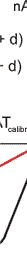
2.6.3 Calibration of the optical detection system

Having got a notion about the relation between the lateral forces and cantilever deformations (see derivation), let us discuss the calibration of the detection unit. Tilts a and b of the cantilever mirrored side result in the reflected laser beam deflection. The laser spot that strikes a photodetector moves along corresponding perpendicular axes a and b (Fig. 1).

(2)

where L – optical "arm" (distance between mirror and the photodiode). The nonzero beam vertical bending ( ) leads to the spot travel in the a direction which produces DFL signal while torsion ( ) – to the travel in the b direction and signal LAT appearance.

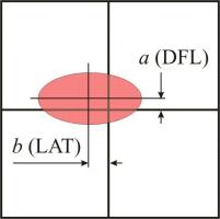
Fig. 1. Spot displacement on the photodetector.

Let us introduce constants of proportionality A, B [nA/mm] between a and DFL, b and LAT:

(3)

We have to admit that the spot in the photodetector plane can be noncircular and have irregular shape and even irregular intensity. This originates from the focusing inaccuracy, laser beam diffraction on the cantilever mirrored surface, etc. Nevertheless, at small displacements a and b (which is true in practice), corresponding signals DFL and LAT are linear in accordance with (3).

Thus, A and B are the constants of the instrument with the specific cantilever installed. One can determine them by performing the needed calibration procedure that will allow to calculate the spot displacement on the photodiode knowing the signals DFL and LAT. For that, it is necessary to measure signals amplitude at known displacements a and b. To produce the known (adjustable) displacements, it is more convenient to move the photodiode rather than deflect the beam (as in case of the cantilever deformation) that is to use the adjustment screws of the photodiode.

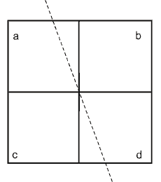
Align the beam – it should strike the photodiode reflecting off the non-deflected cantilever. Using the photodiode adjustment screws, move it along perpendicular axes (Fig. 2) x and h registering signals DFL and LAT after every turn.

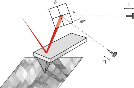
Fig. 2. Optical detection system.

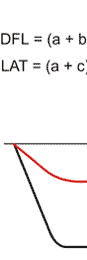
Thus plot relations DFL(x), LAT(x) and DFL(h), LAT(h). Fig. 4 shows the first of them.

Select a interesting region of Fig.3 using mouse pointer.


Fig. 3. Ideal relations DFL(x), LAT(x).										Fig. 4. Location of laser beam spot on photodetector corresponding selected ragion of Fig. 4.

A linear signals variation near zero point turns gradually into a plateau which correspond to a complete spot shift into one of the photodiode segments. When the spot oversteps the diode limits, signal amplitude starts to decrease. This is an ideal case. In practice, plots look more complicated due to the spot irregularity (see Appendix II).

Now, determine what spot displacements in the photodiode co-ordinates (axes a and b) are produced by screws x and h move. Let us find, for example, the change in coordinate a of the spot upon the photodiode move by distance x along the same axis. Not taking into consideration the actual axes direction, suppose that in Fig. 5 the beam strikes the photodiode vertically (beam is always orthogonal the diode) and axis x of the diode move is directed arbitrarily. Points OO'D form a right triangle.

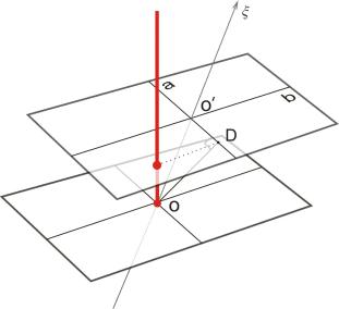
Fig. 5. On expressions (4 - 5).

Then,

(4)

and similarly

(5)

Angles , , , depend on the microscope optical system design and are given in Appendix II.

Having got four relations of (4–5) type, it is possible to "rescale" horizontal axes of plots in Fig. 3. Slope ratio of plots linear portions are calibration constants A and B. Generally, to perform signals LAT and DFL calibration, a couple of plots (one for DFL, the other for LAT) and two of mentioned angles are enough. However, for some microscope models one or two (of four) plots can degenerate into a horizontal line that makes calibration impossible (see example in Appendix II DFL(h) = 0).

Finally, to relate the measured signal with a lateral force acting in the x-direction, expressions (1)–(5) are combined to give

(6)

where calibration constant B is determined as shown above, for example, from the slope of the LAT(x) plot linear portion (Fig. 3):

(7)

Quantitative estimates of the constant B and coefficient of arbitrary units used in LFM conversion into force units are presented in Appendix II.

Summary.

To measure the lateral force, it is necessary to calibrate the microscope optical detection system that allows for the LAT signal conversion into corresponding force.
Calibration is performed using the photodiode adjusting screws. For calculations, one should know cantilever characteristics and employ reference data on microscope Solver P47 various models design, given in Appendix I.