


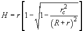
2.5.2 Effect of the tip curvature radius and cone angle
Despite the ability to reach high spatial resolution, the acquired surface topography image can sometimes not correspond to the real surface features due to the effect of the instrument on the object resulting in the artifacts appearance. These artifacts, as a rule, can be easily taken into consideration while qualitatively interpreting the AFM results; however, some special problems can require quantitative estimation and reconstruction of sample true geometry. During scanning, two major AFM artifacts can appear: "profile broadening" effect due to the tip-sample convolution and "height lowering" effect due to the elastic deformation of studied objects. The last effect is considered in detail in chapter 2.5.1. In this chapter the elementary tip-sample convolution phenomenon is examined for the AFM operating in the contact mode. Different tip and sample feature sizes are considered.
1. Tip radius
 is much less than the feature curvature radius
 –
–
 .
.
Fig. 1 depicts the studied object and conical tip geometry in case
.
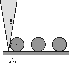
Fig. 1. Schematics of the studied object
and conical tip in case .
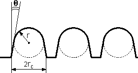
Fig. 2. Image profile of objects shown in Fig. 1.
From the case analysis it easily follows that the object lateral width is:

(1)
where
 – the cone half angle. The corresponding surface profile in the contact mode under given conditions is shown in Fig. 2. In this case, the object is broadened by
 while its height remained the same –
 .
.
2. Tip radius
is approximately equal to the feature curvature radius
–
 .
.
The tip and studied object geometry when
are shown in Fig. 3.
Fig. 3. Schematics of the studied object and conical tip
in case
. Dotted line represents the tip path.
Fig. 4. Image profile of objects shown in Fig. 3.
In this case, the tip move across the object surface can be approximated by the sphere of radius
move along the sphere of radius
surface, i.e. the tip describes arc of radius
 . Elementary calculation gives in this case for the object lateral dimension

(2)
and for the relative height of the object
(3)
If minimum distance between features
 is less than the tip diameter
 (Fig. 3), then, during the tip passing between them, it will penetrate as deep as
(4)
Quantities
 and
and
 are shown in Fig. 4 where the surface image profile is depicted for the given conditions taking into consideration the tip-sample convolution. In this case, the object broadening value is
 . Moreover, the tip finite size does not allow it to penetrate into narrow cavities on the sample surface resulting in their depth and width decrease.
3. Lateral resolution of an AFM.
The resolution criteria in the normal direction
 can be the minimum Z-coordinate change during scanning which can be detected at a given noise level. Resolution depends much on scan parameters (speed, scan size, parameters of the feedback circuit proportional and integration sections) as well as on the sample elastic properties. Normally, the vertical resolution is several tenths of an angstrom.
There is no unambiguous procedure of the microscope lateral resolution determination. The most simple way to estimate it is as follows.
Let
be the probing tip curvature radius and
– resolvable surface feature radius (Fig. 5). Then lateral resolution is connected with the vertical resolution limit
. The resolution criteria is the ability to detect the difference in the tip vertical coordinate over features and between them.
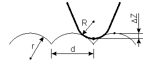
Fig. 5. On defining the lateral resolution:
– vertical resolution limit,
 – desired lateral resolution limit,
and
– curvature radii of tip and resolved objects.
– desired lateral resolution limit,
and
– curvature radii of tip and resolved objects.
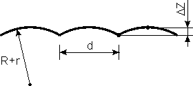
Fig. 6. Expected result of AFM topography study of
surface shown in Fig. 5.
The geometrical analysis (Fig. 5) allows to obtain the expression for the minimum separation between resolved asperities when the AFM image "dip" can still be detected (i.e. equal to the limit
):
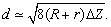
(5)
Because the best spatial resolution must be the invariant characteristic of the instrument (independent on the studied object), it should be defined, e.g. from the condition of two point objects (
 ) detection. Then formula (5) is written as

(6)
relating lateral resolution limit
, vertical resolution limit
and tip curvature radius
.
Summary.
- To reconstruct the sample true geometry one should solve the inverse problem of tip-sample convolution.
- If
, the feature size in the image is defined by formula (1).
- If
, the feature size in the image is defined by expressions (2–4).
- The best lateral resolution in the contact mode depends on the vertical resolution limit (quoted AFM characteristic) and tip curvature radius (6).